DeFi Funding Rate Arbitrage 2026: Perpetual Plays & Tools

Introduction to Funding Rate Arbitrage in DeFi

Funding rate arbitrage has emerged as a sophisticated strategy for generating consistent yields in decentralized perpetual futures markets. As we move into 2026, traders are leveraging long-short funding plays across protocols to exploit rate discrepancies while minimizing directional risk. This approach allows participants to earn from the funding payments themselves rather than relying solely on price movements. Perpetual futures differ from traditional contracts by using funding rates to keep prices aligned with spot markets. When rates turn positive, longs pay shorts; the reverse occurs when rates are negative. Arbitrageurs position accordingly to capture these payments repeatedly, often achieving annualized yields in the mid-teens to low-thirties percent depending on market conditions.

The appeal lies in its market-neutral nature. Unlike directional trading, funding arbitrage profits from the structural imbalance between long and short interest across venues. In 2026, with increased institutional participation and improved cross-chain infrastructure, opportunities have multiplied, but so have the complexities of execution.

Mechanics of Long-Short Funding Plays

Understanding the core mechanics is essential. A typical setup involves opening a long position on one venue and a short on another, or within the same protocol if supported. The goal is to hold both legs until funding settles in your favor. For instance, if a market shows persistently positive funding, the arbitrageur shorts the perpetual and hedges with a spot long position. Funding payments are calculated periodically, typically every hour or eight hours, based on the difference between the perpetual price and the spot index. A concrete example: suppose BTC perpetual funding on one platform averages +0.04% per interval while another shows +0.01%. An arbitrageur can short the higher-rate venue and long the lower-rate venue, pocketing the net 0.03% differential each period after fees.

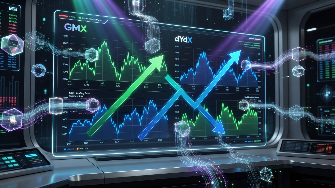
Multi-protocol setups amplify opportunities. Platforms like GMX and dYdX often display divergent rates due to differences in liquidity, user bases, and leverage availability. Traders monitor these spreads in real time to enter when the differential exceeds transaction costs. Advanced players also factor in basis risk between spot and perpetual legs, adjusting hedge ratios dynamically as volatility spikes.

Platform Comparisons: GMX vs dYdX and Beyond

GMX operates on Arbitrum and Avalanche with its unique GLP liquidity model, offering deep liquidity for major pairs. dYdX, now on its own chain, provides high throughput and competitive funding dynamics. Key differences include fee structures, supported assets, and oracle mechanisms. GMX tends to favor longer holding periods for funding capture, while dYdX suits high-frequency adjustments.

Traders should evaluate liquidation thresholds and margin requirements across venues before scaling positions. Additional considerations include oracle reliability, maximum leverage caps, and historical funding rate stability. GMX’s GLP pool provides single-sided liquidity advantages but introduces slight impermanent loss exposure, whereas dYdX’s order book model offers more precise entry pricing. Comparing these venues side-by-side helps identify which markets consistently produce the most attractive funding spreads for arbitrage.

Real-Time Monitoring with On-Chain Data Tools

Effective arbitrage demands robust monitoring. On-chain analytics platforms provide dashboards for funding rates, open interest, and historical spreads. Integrating these with wallet alerts enables rapid response to shifting conditions. Popular tools aggregate data from multiple chains, allowing users to compare GMX funding against dYdX equivalents instantly. Custom scripts using blockchain indexers can automate alerts when rates breach predefined thresholds.

Professional traders often combine multiple data sources, including subgraph queries and WebSocket feeds, to build comprehensive views of funding velocity and predicted next payments. This real-time visibility is critical because funding rates can flip within minutes during high-volatility events.

Step-by-Step Example: Spotting and Executing an Opportunity

1. Scan funding rate dashboards across protocols for divergences exceeding 0.05% hourly.
2. Verify liquidity depth to ensure slippage remains minimal on both legs.
3. Calculate expected net yield after all fees and gas costs using a spreadsheet model.
4. Open the short leg on the high-funding venue and the long hedge on spot or the opposing perpetual.
5. Set stop-losses based on volatility bands to protect against sudden rate reversals.
6. Monitor and rebalance every 4-8 hours as rates evolve, documenting each funding collection.

Risk Controls for Volatility and Liquidation Cascades

Volatility poses the primary threat. Sudden market moves can trigger liquidations even in hedged positions if leverage is too high. Best practice involves capping total leverage at 2-3x and maintaining excess collateral buffers. Liquidation cascades occur when cascading margin calls amplify price swings. Diversifying across uncorrelated pairs and using isolated margin modes helps mitigate this. Always simulate scenarios with historical data before live deployment. Additional safeguards include setting automated alerts for funding rate spikes above 0.1% per interval and maintaining a reserve of stablecoins for rapid margin top-ups during flash events.

Gas Optimization Across Chains

Arbitrage profits erode quickly under high gas fees. Strategies include batching transactions during low-fee windows, using Layer-2 solutions like Arbitrum for GMX trades, and employing meta-transactions where supported. Cross-chain bridges should be evaluated for both cost and speed. In practice, routing through optimized aggregators and scheduling larger position adjustments during off-peak hours can reduce effective gas costs by 40-60% compared to naive execution.

Integration with Broader DeFi Strategies

Funding arbitrage pairs well with yield farming and options overlays. Yields from funding can be reinvested into liquidity pools, compounding returns. Some advanced users combine it with delta-neutral vaults for automated execution. This integration allows traders to stack multiple yield sources while keeping overall portfolio delta near zero, enhancing capital efficiency in a maturing DeFi ecosystem.

Common Pitfalls to Avoid

• Ignoring cumulative fees that turn marginal edges negative.
• Over-leveraging during low-volatility periods leading to unexpected liquidations.
• Failing to account for oracle delays that misalign funding calculations.
• Neglecting tax reporting requirements on realized funding income.
• Underestimating bridge and withdrawal times when moving collateral between chains mid-trade.

FAQs on Tax Implications and Automation

How are funding payments taxed? Funding income is typically treated as ordinary income in most jurisdictions. Consult a crypto-savvy tax professional for your specific location.

Can keepers automate passive execution? Yes, keeper networks and custom bots can monitor rates and adjust positions automatically, though they introduce smart contract risks.

What minimum capital is realistic? Start with amounts sufficient to cover fees and maintain safe margins, often several thousand USD equivalent depending on the chain.

How do liquidation cascades impact hedged positions? Even hedged setups can face temporary margin shortfalls if one leg liquidates first. Using lower leverage and isolated margin reduces cascade exposure.

By mastering these elements, traders position themselves for sustainable yields in the evolving 2026 DeFi landscape. Always verify current protocol parameters directly on GMX and dYdX before trading.